ALBuMS pipeline tutorial

This notebook is a hands-on tour of the ALBuMS architecture and workflow rather than a physics benchmark (see the other notebooks in examples/ and benchmark_aladdin/ for physics-result demonstrations). ALBuMS predicts various instabilities in double-RF storage rings through a three-stage pipeline:

1. Equilibrium (albums.equilibrium) — solve the beam’s longitudinal equilibrium (bunch profile, bunch length, form factors, Touschek lifetime ratio, xi) for a given ring, cavity list and beam current. Three equilibrium solvers are available (Bosch, Venturini, Alves), each providing a different subset of derived quantities.

2. Theories (albums.theories) — given a solved equilibrium, evaluate a chosen subset of instability theories (zero-frequency, Robinson, HOM-driven coupled-bunch, PTBL, …). Each theory only needs some of the equilibrium’s derived quantities.

3. Flow / Result (albums.flow) — a Flow ties one equilibrium solver to a list of theories; SystemState.run(flow, ...) solves the equilibrium then evaluates the flow’s theories, returning a structured Result.

Not every theory is compatible with every solver (e.g. the Bosch solver does not compute the phase form factor that the PTBL criteria need) — this is expressed as a set of capabilities and checked automatically before any computation runs.

We walk through all three stages, then scale Stage 3 up to a full 2D parameter scan and plot the result. The running example is the Aladdin storage ring (standard lattice, passive harmonic cavity — the same setup used throughout the test suite and the benchmark_aladdin/ notebooks).

1. Build a ring and cavities

ALBuMS operates on mbtrack2 objects: a Synchrotron ring and a list of CavityResonator cavities (main cavity first, then one or more harmonic cavities).

import numpy as np
from scipy.constants import c
from mbtrack2 import Electron, Optics, Synchrotron, CavityResonator

h = 15
L = 2.96e-7 * c
E0 = 0.8e9
particle = Electron()
ac = 0.0335
tau = np.array([None, None, 13.8e-3])
U0 = 17.4e3
tune = np.array([None, None])
emit = np.array([None, None])
sigma_0 = 250e-12
sigma_delta = 4.8e-4
chro = [0, 0]

optics = Optics(
    local_beta=np.array([1, 1]),
    local_alpha=np.array([0, 0]),
    local_dispersion=np.array([0, 0, 0, 0]),
)

ring = Synchrotron(
    h, optics, particle,
    L=L, E0=E0, ac=ac, U0=U0, tau=tau,
    emit=emit, tune=tune,
    sigma_delta=sigma_delta, sigma_0=sigma_0, chro=chro,
)
ring.f1 = 50600000.0
V_RF = 90e3
tuneS = ring.synchrotron_tune(V_RF)
ring.sigma_0 = ring.sigma_delta * np.abs(ring.eta()) / (tuneS * 2 * np.pi * ring.f0)

# Main cavity (m=1) — driven by its generator.
MC = CavityResonator(ring, m=1, Rs=0.5e6, Q=8000, QL=8000, detune=100e3)
MC.beta = 11
MC.Vc = 90e3
MC.theta = np.arccos(ring.U0 / MC.Vc)

# Passive harmonic cavity (m=4) — beam-driven, used for bunch lengthening.
HC = CavityResonator(ring, m=4, Rs=1.24e6, Q=20250, QL=20250, detune=100e3)

2. Stage 1 — SystemState and the beam equilibrium

SystemState bundles the ring and the cavity list. The cavities are deep-copied, so solving never mutates the objects you passed in. Every solver option — the beam current, the integration boundary, and all solver-specific flags — lives in a single frozen EquilibriumOptions dataclass.

run_equilibrium runs only Stage 1: useful when you only care about bunch profile, bunch length, the Touschek lifetime ratio or xi and want to skip the instability theories entirely. (It still takes a flow, to know which equilibrium solver to use; the flow’s theory list is ignored here.)

from albums import SystemState, EquilibriumOptions, DEFAULT_FLOWS

system = SystemState(ring, [MC, HC])
eq_opts = EquilibriumOptions(I0=0.1)  # 100 mA

eq_result = system.run_equilibrium(DEFAULT_FLOWS["Venturini"], eq_opts)
eq = eq_result.equilibrium

print("converged:", eq_result.converged)
print("bunch_length [ps]:", eq.bunch_length * 1e12)
print("amplitude form factor F:", eq.F)
print("Touschek lifetime ratio:", eq.Touschek, " xi:", eq.xi)
print("capabilities:", sorted(c.value for c in eq.capabilities))

converged: True
bunch_length [ps]: 350.23712417309866
amplitude form factor F: [0.99381883 0.90538203]
Touschek lifetime ratio: 1.3830383058642555  xi: 0.5078414129893387
capabilities: ['amplitude_form_factor', 'mbtrack2_ble', 'phase_form_factor', 'taylor_potential', 'touschek_lifetime_ratio']

The capabilities set is the key to the whole pipeline: it lists exactly which derived quantities this solver produced. Each instability theory declares which capabilities it requires, so the two can be matched automatically — that is what the Flow below builds on.

3. The Flow concept

A Flow is just (equilibrium_solver, [theories]). DEFAULT_FLOWS provides the ready-made “classic” choices (one equilibrium method + its usual theory subset); you can also build a custom Flow with any solver/theory combination.

Not every combination is valid: each theory declares the Capability set it requires, each solver declares the set it provides, and Flow.validate() (called automatically inside .run()) rejects an incompatible pair before any computation runs. The compatibility matrix below is generated straight from the code.

from albums import compatibility_matrix

print("Default flows:", list(DEFAULT_FLOWS.keys()))
print()
print(compatibility_matrix())

Default flows: ['Bosch', 'Bosch_no_coupling', 'Venturini', 'Alves']

| Theory | Bosch | Venturini | Alves |
|---|:--:|:--:|:--:|
| `zero_frequency` | ✅ | ✅ | ✅ |
| `robinson_coupling` | ✅ | ✅ | ✅ |
| `robinson_no_coupling` | ✅ | ✅ | ✅ |
| `hom_coupled_bunch` | ✅ | ✅ | ✅ |
| `bosch_mode1` | ✅ | ✅ | ✅ |
| `ptbl_he` | ❌ | ✅ | ✅ |
| `ptbl_alves` | ❌ | ❌ | ✅ |
| `robinson_glmci` | ❌ | ❌ | ✅ |

Capability validation in action

PTBLAlves needs the pycolleff longitudinal-equilibrium handle and the full bunch distribution — capabilities only the Alves solver provides. Pairing it with the Bosch solver is invalid, and .run() raises before doing any work:

from albums import Flow, BoschEquilibrium, PTBLAlves, IncompatibleFlowError

bad_flow = Flow(BoschEquilibrium(), [PTBLAlves()])
try:
    system.run(bad_flow, eq_opts)
except IncompatibleFlowError as exc:
    print(exc)

Flow 'custom' is invalid:
  - theory 'ptbl_alves' needs [full_distribution, pycolleff_le] which 'Bosch' does not provide

4. Stages 2 + 3 — running a Flow and reading the Result

.run(flow, eq_opts, theory_opts) solves the equilibrium (Stage 1) then evaluates every theory in the flow (Stage 2), returning a structured Result (Stage 3). theory_opts carries the inputs shared across theories (HOM parameters, …).

The Result exposes flow-agnostic accessors — the same names work whatever solver and theory list the flow used, so downstream code never has to special-case the method.

from albums import TheoryOptions

theory_opts = TheoryOptions(mode_coupling=True)
result = system.run(DEFAULT_FLOWS["Venturini"], eq_opts, theory_opts)

print("converged:", result.converged)
print("theories evaluated:", list(result.theories.keys()))
print()
print("zero_frequency unstable:", result.zero_frequency)
print("robinson_flags (dipole..octupole):", result.robinson_flags)
print("PTBL unstable:", result.ptbl)
print("HOM unstable:", result.hom)
print("any_unstable:", result.any_unstable)
print()
print("Touschek lifetime ratio:", result.Touschek)
print("bunch_length [ps]:", result.equilibrium.bunch_length * 1e12)

converged: True
theories evaluated: ['zero_frequency', 'robinson_coupling', 'hom_coupled_bunch', 'ptbl_he']

zero_frequency unstable: False
robinson_flags (dipole..octupole): [False False False False]
PTBL unstable: False
HOM unstable: False
any_unstable: False

Touschek lifetime ratio: 1.3829757033254442
bunch_length [ps]: 350.2216065105191

Same operating point, several flows

Because every solver/theory combination exposes the same Result shape, switching methods is just swapping which Flow you pass in. Here we run the same ring, cavities and beam current through all of DEFAULT_FLOWS:

print(f"{'flow':<18} {'converged':<10} {'Touschek lifetime ratio':>20} {'bunch_length [ps]':>20} {'any_unstable':>14}")
for name, flow in DEFAULT_FLOWS.items():
    r = system.run(flow, eq_opts, theory_opts)
    print(f"{name:<18} {r.converged!s:<10} {r.Touschek:>20.4f} "
          f"{r.equilibrium.bunch_length * 1e12:>20.3f} {r.any_unstable!s:>14}")

flow               converged  Touschek lifetime ratio    bunch_length [ps]   any_unstable
Bosch              True                        nan              348.487          False
Bosch_no_coupling  True                        nan              348.487          False
Venturini          True                     1.3829              350.200          False
Alves              True                     1.3781              349.140          False

5. Stage 3 at scale — a parameter scan

A single .run() gives one operating point. To map a region of parameter space you use the scan functions in albums.scan. Each scan:

• takes a SystemState, two swept axes, a flow, and the typed *_opts;

• calls SystemState.run(...) at every grid point (mutating the relevant cavity attribute);

• returns a self-describing ResultArray that carries its own axes, display units, axis labels and the flow — so plotting needs no further arguments. Scans never name or save anything: persist a result explicitly with result.save(name) (§7).

Scans are MPI-parallelized: the outer axis is split across ranks with np.array_split, so for a real sweep you launch

mpirun -n <N> python your_scan_script.py

Any rank count works (a rank may own 0+ rows). Inside this notebook we just run single-process, which is fine for a small grid.

Here we use scan_psi_I0, which sweeps the harmonic-cavity tuning angle psi_HC (in degrees, the outer axis) against the beam current (the inner axis).

from albums import scan_psi_I0

psi_HC_vals = np.linspace(80, 90, 25)     # harmonic-cavity tuning angle [deg]
currents = np.linspace(0.02, 0.3, 25)     # beam current [A]

scan_eq_opts = EquilibriumOptions()       # note: no I0 — the scan fills it per point

result = scan_psi_I0(
    SystemState(ring, [MC, HC]),
    psi_HC_vals,
    currents,
    flow=DEFAULT_FLOWS["Bosch"],
    eq_opts=scan_eq_opts,
    theory_opts=theory_opts,
)

print("grid shape (psi_HC x current):", result.shape)
print("flow:", result.flow)

scan:   0%|          | 0/625 [00:00<?, ?it/s]

scan:   2%|▏         | 14/625 [00:00<00:04, 139.74it/s]

scan:   4%|▍         | 28/625 [00:00<00:04, 123.14it/s]

scan:   7%|▋         | 46/625 [00:00<00:03, 147.27it/s]

scan:  10%|█         | 63/625 [00:00<00:03, 155.64it/s]

scan:  13%|█▎        | 79/625 [00:00<00:03, 141.80it/s]

scan:  16%|█▌        | 99/625 [00:00<00:03, 158.11it/s]

scan:  19%|█▉        | 120/625 [00:00<00:02, 173.41it/s]

scan:  23%|██▎       | 141/625 [00:00<00:02, 183.92it/s]

scan:  26%|██▌       | 164/625 [00:00<00:02, 196.80it/s]

scan:  30%|███       | 188/625 [00:01<00:02, 207.83it/s]

scan:  34%|███▍      | 211/625 [00:01<00:01, 213.74it/s]

scan:  37%|███▋      | 233/625 [00:01<00:01, 203.91it/s]

scan:  41%|████      | 255/625 [00:01<00:01, 205.91it/s]

scan:  44%|████▍     | 276/625 [00:01<00:01, 206.79it/s]

scan:  48%|████▊     | 297/625 [00:01<00:01, 206.80it/s]

scan:  51%|█████     | 318/625 [00:01<00:01, 203.95it/s]

scan:  54%|█████▍    | 339/625 [00:01<00:01, 202.85it/s]

scan:  58%|█████▊    | 360/625 [00:01<00:01, 201.67it/s]

scan:  61%|██████    | 381/625 [00:02<00:01, 198.81it/s]

scan:  64%|██████▍   | 403/625 [00:02<00:01, 202.62it/s]

scan:  68%|██████▊   | 424/625 [00:02<00:00, 201.99it/s]

scan:  71%|███████   | 445/625 [00:02<00:00, 195.96it/s]

scan:  74%|███████▍  | 465/625 [00:02<00:00, 196.82it/s]

scan:  78%|███████▊  | 485/625 [00:02<00:00, 192.83it/s]

scan:  81%|████████  | 505/625 [00:02<00:00, 193.45it/s]

scan:  84%|████████▍ | 525/625 [00:02<00:00, 190.21it/s]

scan:  87%|████████▋ | 545/625 [00:02<00:00, 185.30it/s]

scan:  90%|█████████ | 564/625 [00:02<00:00, 183.25it/s]

scan:  93%|█████████▎| 583/625 [00:03<00:00, 177.45it/s]

scan:  96%|█████████▌| 601/625 [00:03<00:00, 172.23it/s]

scan:  99%|█████████▉| 619/625 [00:03<00:00, 171.25it/s]

scan: 100%|██████████| 625/625 [00:03<00:00, 186.35it/s]

grid shape (psi_HC x current): (25, 25)
flow: Flow(equilibrium=BoschEquilibrium(), theories=[ZeroFrequency(), RobinsonCoupling(), HOMCoupledBunch(), BoschMode1()], name='Bosch')

6. Reading and plotting the ResultArray

A ResultArray is the grid-level analogue of Result: the same flow-agnostic accessors, now returning 2D numpy arrays over the (psi_HC, current) grid. Missing or non-converged points read back as sentinels (NaN for floats, False for flags).

print("xi array shape:", result.xi.shape)
print("Touschek lifetime ratio array shape:", result.Touschek.shape)
print("bunch_length array shape:", result.bunch_length.shape)
print("fraction of grid converged:", result.converged.mean())
print("fraction of grid unstable:", result.any_unstable.mean())
print()
# One grid point as a nested dict (no Result object rebuilt):
pt = result.point((0, -1))   # lowest tuning angle, highest current
print("point (0, -1) bunch_length [ps]:", pt["equilibrium"]["bunch_length"] * 1e12)

xi array shape: (25, 25)
Touschek lifetime ratio array shape: (25, 25)
bunch_length array shape: (25, 25)
fraction of grid converged: 1.0
fraction of grid unstable: 0.5648

point (0, -1) bunch_length [ps]: 1275.3569076708275

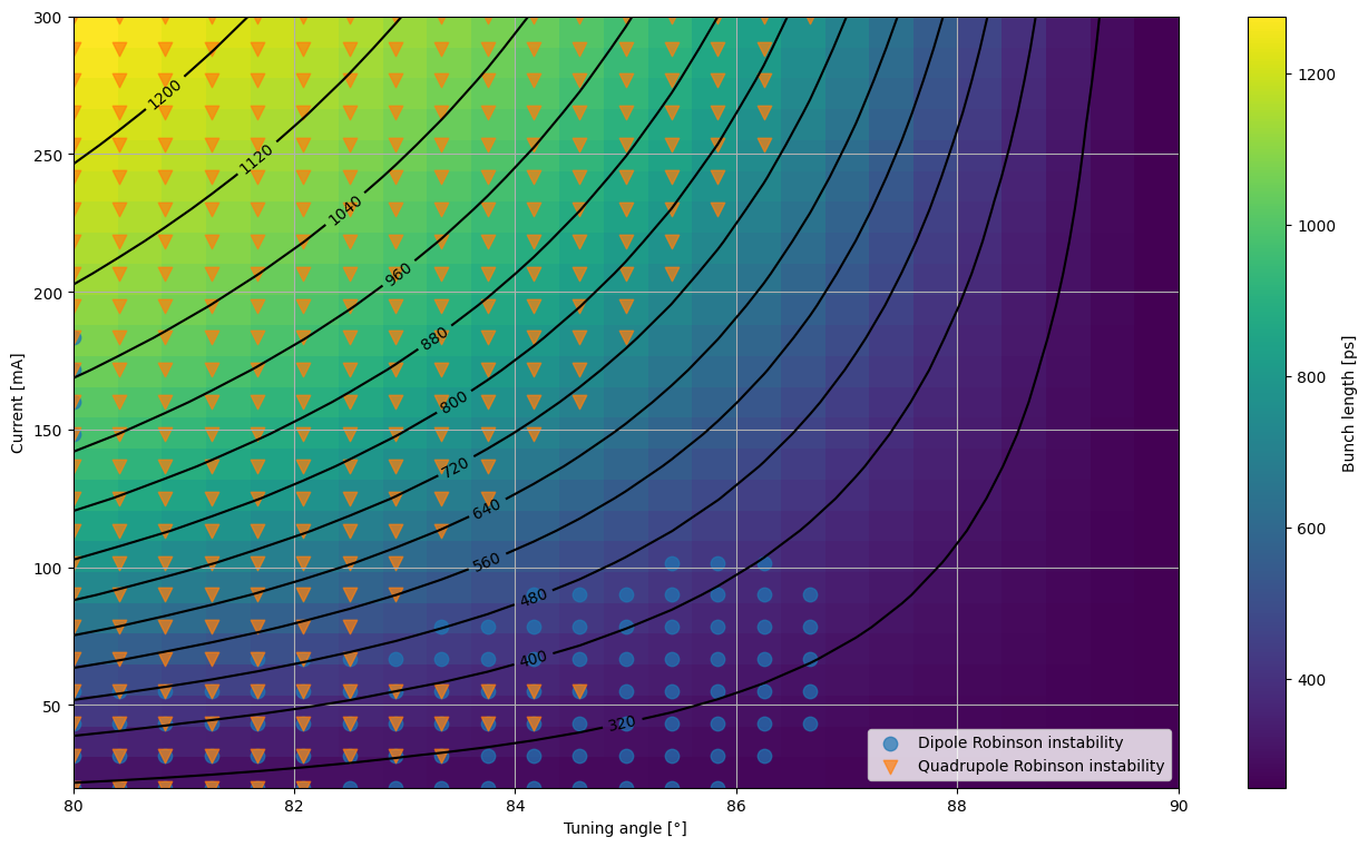
result.plot(quantity) draws one background colour-map quantity plus the instability markers for whatever theories the flow ran — and because the axes, units, labels and flow are stored on the result, no extra arguments are needed.

Valid quantity strings include "xi", "bunch_length", "Touschek" (Touschek-lifetime ratio), "growth" (most-unstable growth rate across all theories) and "growth_<theory_name>" for a single theory. Pass a PlotOptions via plot_opts=... to tweak the colour map, contours, marker size, colour-bar limits, etc.

import matplotlib.pyplot as plt

result.plot("bunch_length")
plt.show()

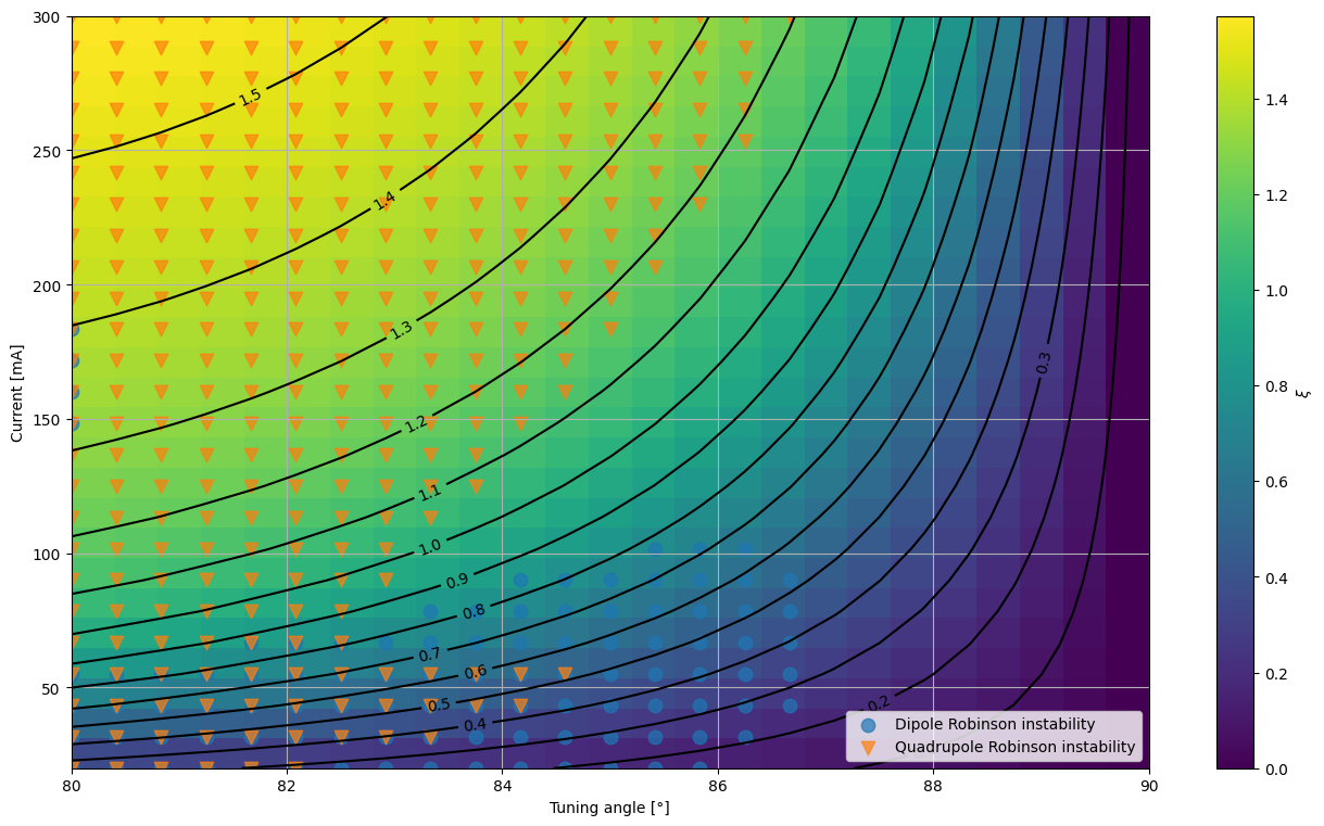
result.plot("xi")
plt.show()

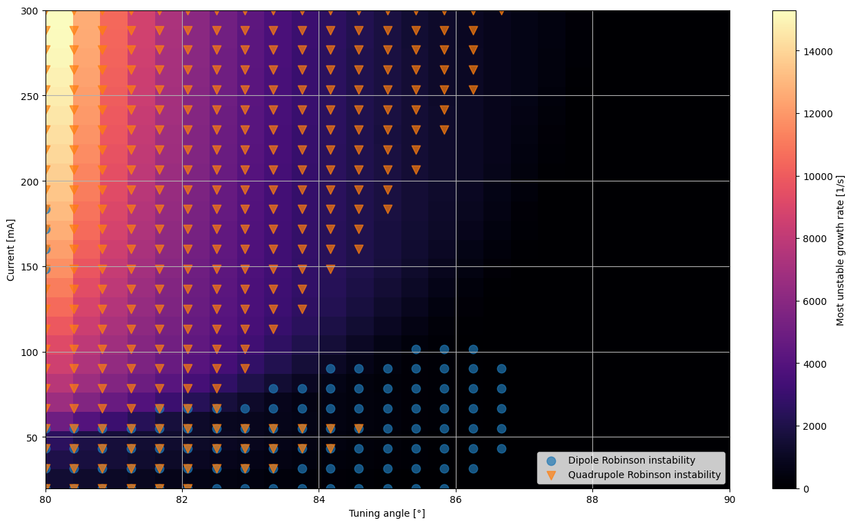
from albums import PlotOptions

# Display tweaks via PlotOptions (here: a different colour map, no contour lines).
result.plot("growth", plot_opts=PlotOptions(cmap="magma", contour=False))
plt.show()

7. Saving and loading a scan

ResultArray.save(name) writes <name>.hdf5 — the full nested grid plus the scan metadata (axes, units, labels, flow). The name is mandatory and is only the file name; it is not stored as a plot title. ResultArray.load(file) reconstructs a fully self-describing object, so a loaded result re-plots with the same one-liner.

import os
from albums import ResultArray

result.save("pipeline_demo")          # -> pipeline_demo.hdf5

reloaded = ResultArray.load("pipeline_demo.hdf5")
print("reloaded shape:", reloaded.shape)
print("reloaded flow:", reloaded.flow)

reloaded.plot("bunch_length")          # same plot, no extra args — metadata survived the round-trip
plt.show()

os.remove("pipeline_demo.hdf5")        # tidy up the tutorial artefact

reloaded shape: (25, 25)
reloaded flow: Bosch

See also

• Other parameter scans in albums.scan: scan_psi_RoQ, scan_psi_QL, scan_psi_MCdet, scan_MC_Vc_HC_Vc_active, … — all return the same ResultArray.

• Optimiser scans (scan_RoQ_I0, scan_RoQ_Q0, …) and albums.optimiser tune the harmonic-cavity angle to maximise the Touschek-lifetime R-factor at each grid point; see examples/SOLEIL_II_optimize_RoQ_Q0.ipynb.

• Physics-result demonstrations: examples/Single_RF_instabilities.ipynb, examples/SOLEIL_II_instability_map.ipynb and the benchmark_aladdin/ notebooks.

• README.md for the same Flow-API story in prose, with albums.compatibility_matrix() as the single source of truth for which theory works with which solver.